Learning design · 2025–2026
EcoGEM
I designed EcoGEM to help my Grade 6 students explain how changes move through an ecosystem. It brings together a guided investigation and an interactive lab where students can build food webs, test predictions, and revise their thinking.
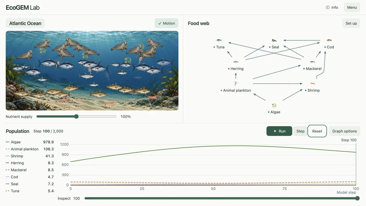
From a food chain to a connected system
A food chain can make a relationship look simple: one organism eats another. The harder question is what happens elsewhere in the web when that relationship changes.
That is the learning problem behind EcoGEM. I want students to explain indirect effects, notice changes over time, and use evidence to reconsider an idea. The aim is a stronger explanation, not just a web that stays unchanged.
The learning design came first
The original EcoGEM project
My 2025 learning design used the Annenberg Ecology Lab as a space for investigation. I adapted the Generate–Evaluate–Modify (GEM) approach described by Samia Khan: make an explanation, test it, then revise it using the evidence. GEM is the teaching framework I drew on, not a framework I invented. The simulation was the original authors’ work; the guided learning design was mine.
The lab I built for it
When access to the original experience became unreliable, I built EcoGEM Lab with Codex. It is an independent implementation with new illustrations, five ecosystems, a simpler starting setup, and saved A/B experiments. The guided investigation now uses this lab.
EcoGEM is the overall learning project. EcoGEM Lab is its simulation. They share a purpose, but the lab also works on its own, without lesson questions.
What students can investigate
Build a connected web
Start with a simple chain. Add an organism or change an offered feeding link, then predict which populations might respond.
Compare two possibilities
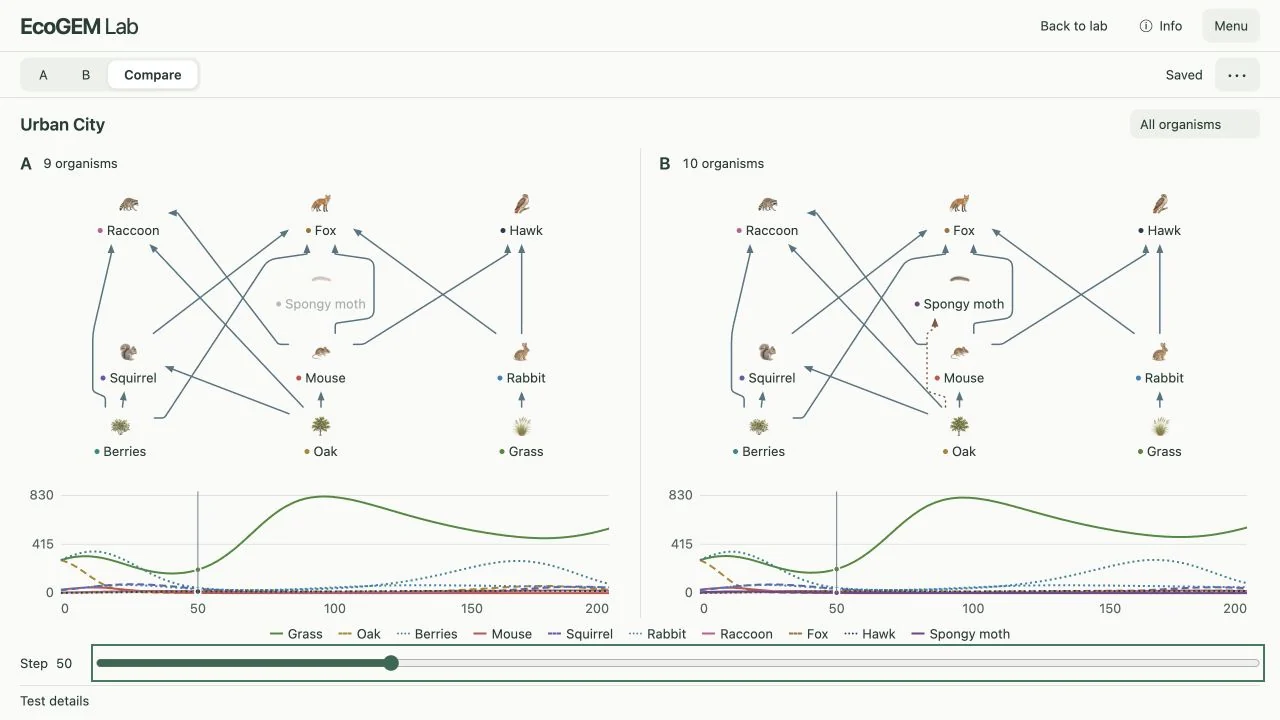
Keep scenario A, change one thing in B, and compare their food webs and graphs at the same model step.
Explore a disturbance
Introduce an invasive species where available. Compare what happens with and without repeated human removal.
Five places to start
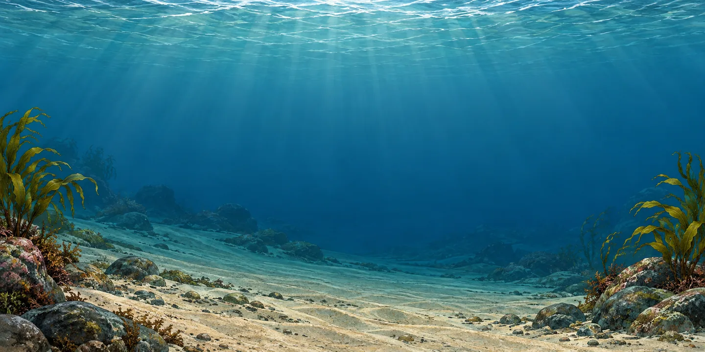
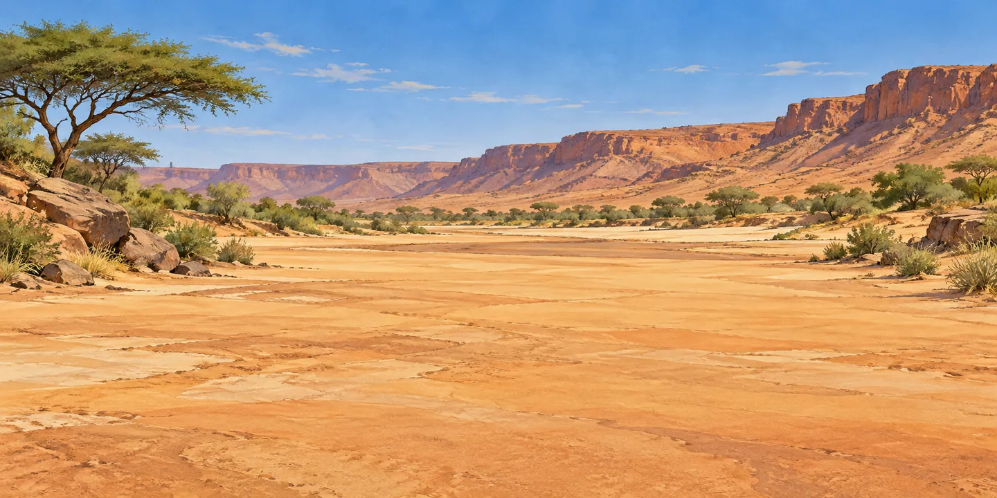
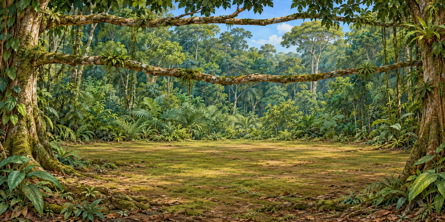
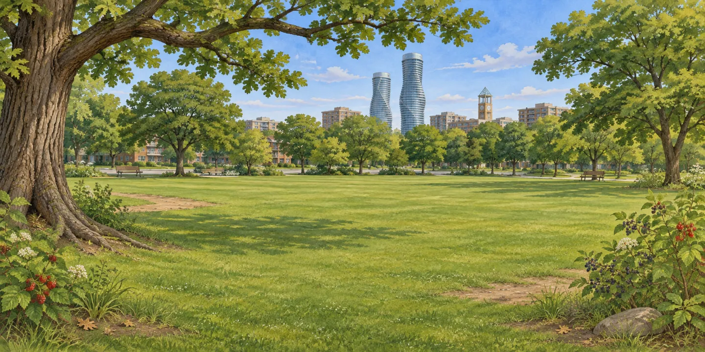
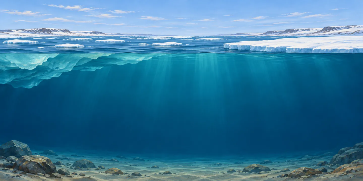
The city is inspired by Mississauga’s parks and ravines. Each ecosystem is a selected teaching example, with a small set of researched feeding relationships.
Two ways to use EcoGEM
Explore the lab
The standalone simulation is for open exploration or a teacher-led discussion. It has the food web, habitat, and graph, without a question sheet.
Follow the guided investigation
The same lab appears above a notebook for predictions, observations, and revised explanations. Notes stay on the device and can be downloaded.
Trying it with your family? Choose Urban City, then Set up · Simple chain. Predict what adding Hawk might change before pressing Play. Use the web and graph to talk about what surprised you.
Teaching with it? My teacher guide includes lesson openings, experiment setups, discussion prompts, and assessment ideas linked to Ontario’s Grade 6 curriculum.
Read more
Teaching approach, curriculum & original design
Begin with a short orientation so students can use the three views. Then move through competition, connected food webs, and disturbance. Each investigation adapts Khan’s Generate–Evaluate–Modify (GEM) approach: make a prediction, compare it with evidence, and revise the explanation.
This sequence supports Ontario’s Grade 6 Science and Technology curriculum, especially B2.5 (ecological interrelationships) and A1.2/A1.5 (investigation and communication). It offers discussion of biodiversity and resilience, with an Ontario spongy-moth investigation and further local research. It does not cover the entire biodiversity strand. Read the official curriculum
Open the full EcoGEM experience for the embedded lab and student notebook. The teacher guide includes lesson openings, exact experiment setups, discussion prompts, assessment, access supports, and curriculum connections. Download the guide as a PDF.
The GEM framework
Khan, S. (2011). New pedagogies on teaching science with computer simulations. Journal of Science Education and Technology, 20(3), 215–232. https://doi.org/10.1007/s10956-010-9247-2
The article was first published online in September 2010, the year cited in my original paper; the journal issue is dated 2011.
The original design paper
I developed the original EcoGEM learning design in 2025 during my Master of Educational Technology studies at the University of British Columbia. It explains the learning problem, research rationale, and Generate–Evaluate–Modify sequence. It records the earlier experience and includes screenshots of the original Annenberg lab.
Read my original EcoGEM design paper (PDF). The current screenshots and tools on this page show how the project has developed since then.
How the model works & where the numbers come from
I built this lab with Codex, OpenAI’s coding assistant. I directed the learning goals and design; Codex implemented the equations and selected the numerical parameters for classroom exploration. The model uses established ecological ideas: logistic-style producer growth, saturating predator–prey feeding, mortality, and crowding. The ecological literature on feeding responses explains the principle of feeding that levels off as prey becomes abundant; it does not supply or validate this lab’s particular numbers.
The feeding sources below support the selected relationships, not their simulated strength, timing, or population sizes. Codex’s parameter choices were not fitted to measurements of these organisms. The outcomes illustrate possibilities within a simplified teaching model, not predictions about real ecosystems. A changing or declining starting web is something to investigate, not a failed score.
Model steps and abundance units are illustrative. Real species vary by location, season, life stage, and influences that are absent here.
Producers grow toward a resource limit. Consumers feed on their selected prey, gain a fraction of the food they consume, and lose abundance through mortality and crowding. Feeding saturates as food becomes plentiful. The resource slider changes the producer carrying capacity; its rainfall, nutrient, plant-productivity, and algal-productivity labels are conceptual, not measurements. The Arctic control does not simulate sea-ice loss.
Plant abundance represents available food such as leaves, fruit, seeds, and plankton. It does not mean that a tree dies each time an animal eats a leaf. The habitat uses layered depth, gentle movement, and shadows on a single canvas. Motion can be switched off and respects reduced-motion preferences. Positions and movement are illustrative, not simulated animal behaviour. Each species uses a fixed drawing scale, so its visible abundance rises and falls with its graph values; a partially faded portrait represents part of a drawing unit. Portraits are not to scale and their counts are capped for readability. I use the graph for exact model values.
Equations and reproducibility
Producer growth is rᵢNᵢ(1 − (Nᵢ + 0.35ΣNother producers) / (K × resource)), before consumption. Consumers request prey at aᵢNᵢNⱼ / (hᵢ + ΣNselected prey). Shared requests cannot exceed the prey available in that substep. Consumer growth is eᵢ × food consumed − mᵢNᵢ − cᵢNᵢ².
The engine uses 20 simultaneous substeps per model step. Abundance below 0.1 is treated as extinction, and an extinct species returns only when deliberately reintroduced. Runs stop at step 2,000. The same setup and changes produce the same result; the model contains no random events.
Changing a web pauses the simulation and records the intervention. Reset starts the current web again with the chosen starting abundances. A new preset starts a fresh web with its preset values. The other scenario is preserved. CSV contains every step’s abundances; the experiment JSON also contains the initial state, settings, intervention states and model version. A paired download keeps both complete scenarios.
Parameter values are educational choices, not measurements fitted to these organisms. I did not reproduce the original Ecology Lab’s mathematical engine. Its publicly available calculation code uses a different feeding equation and competition settings, so this model will not reproduce historical worksheet values.
Controls, saved experiments & optional support
In the food web’s Set up menu, I can choose a Simple chain, a Small food web, the Full ecosystem, Producers only, or Build your own. I can add organisms and edit their offered feeding links as the question develops. Selecting a preset starts the current scenario at step 0 and leaves the other scenario saved.
I enable Menu · Teacher controls · Edit starting values, then click a species in the food web and open Starting amount at the bottom of its details. I can edit it only at step 0. Reset keeps the values I chose; restoring a preset returns to that preset’s starting values. These are model units, not estimates of wild populations.
I move across the graph to see the step and population beside the thin line. Nothing locks when I click. On a phone I can drag. Excluded organisms are omitted from the graph and its value list, while their recorded history remains in downloads. Excluding a species also changes the food web; it is not just a display filter.
All five ecosystems save separately in my browser. There is no sign-up, and the lab sends no experiment data to a server. Menu · Experiments opens a separate A / B / Compare workspace. Each scenario keeps its own setup, changes and full results. I can copy a starting setup or branch from the current step, then compare their food webs and all included organisms on matching graph axes. A shared slider moves both inspection lines together; on my phone, I open either food web when I need it. I can download both scenarios together.
Optional support
I use the same model for both modes. Guided mode offers optional descriptions of recent patterns and a shaded graph interval. Independent mode leaves interpretation to the learner. Teacher controls in the lab’s Menu let me reveal or hide individual hint types without resetting an experiment.
Hints describe up to 50 recent steps and restart their window after an intervention. They distinguish increasing, decreasing, fluctuating, settling, changing little, zero abundance, and excluded organisms. They are teaching heuristics, not a stable/unstable judgement or proof of causation. Ecological stability has several meanings, including persistence and recovery after disturbance; see DeAngelis and Xu’s overview.
Feeding-relationship research
I used the following research and species accounts for the selected feeding relationships. These sources establish possible foods, not the model’s rates or predictions. Urban mouse, rabbit, and squirrel links sometimes use broader prey categories with a representative local species. The Arctic is a seasonal regional example, not every species feeding together at one moment.
Atlantic Ocean
- NOAA: Copepods—Cows of the Sea
- Fisheries and Oceans Canada: Northern shrimp
- Yunda-Guarin et al. (2025), Trophic ecology and nutritional status of northern shrimp in Canada’s sub-Arctic
- Suca et al. (2018), Feeding dynamics of Northwest Atlantic small pelagic fishes
- Trophic Ecology of Atlantic Cod off Cape Cod, 2001–2004
- Smithsonian National Zoo: Gray seal
- COSEWIC (2011), Atlantic bluefin tuna assessment
Sahara Desert
- FAO: Desert locust frequently asked questions
- Feedipedia: Desert grass (Panicum turgidum)
- Osborn & Helmy (1980), The contemporary land mammals of Egypt (including Sinai)
- Degen (1988), Ash and electrolyte intakes of the fat sand rat consuming saltbush
- Daly & Daly (1973), On the feeding ecology of Psammomys obesus
- Brahmi et al. (2012), First quantitative data on the diet of the fennec fox in Algeria
- León (2020), Cerastes cerastes—MoroccoHerps
- Cole & Wilson (2015), Felis margarita (Carnivora: Felidae)
- IUCN/SSC Cat Specialist Group: Sand cat
Amazon Rainforest
- New York Botanical Garden: Bertholletia excelsa taxon account
- Julliot & Sabatier (1993), Diet of the red howler monkey in French Guiana
- Wisconsin National Primate Research Center: Red howler monkey
- Aquino & Bodmer (2004), Plantas útiles en la alimentación de primates en la cuenca del río Samiria, Amazonia Peruana
- The demography of a resource specialist in the tropics: Cecropia trees and the fitness of three-toed sloths (2019)
- Sloths like it hot: ambient temperature modulates food intake in the brown-throated sloth (2015)
- Aguiar-Silva et al. (2014), Food habits of the harpy eagle, a top predator from the Amazonian rainforest canopy
- Emmons (1987), Comparative feeding ecology of felids in a neotropical rainforest
Urban City
Arctic Ocean
- Cleary et al. (2017): Calanus glacialis feeding
- Schaafsma et al. (2024): Arctic cod stomach-content study
- COSEWIC (2019): ringed seal food and predators
- COSEWIC (2020): beluga feeding relationships
- Eastern Beaufort Sea beluga foraging research (2021)
- NOAA Fisheries: bowhead whale diet
- Diogou et al. (2023): bowheads in the Canadian Arctic
Invasive-species research & modelling choices
I introduce an invader directly in the food web, using Set up · Invasive species where it is available. Its species card gives a short explanation and an optional human-intervention switch. I make predictions with my class before we use the usual Play button and follow the population graph.
I based these additions on published research about real invasions. Codex selected fictional growth, competition and removal settings to make possible effects visible. Abundances are model units, steps are not days, and the outcomes do not predict what will happen in these places. Human intervention represents repeated removal; observing alone does not remove an invader. Urban City includes spongy moth, an introduced leaf-eating insect documented in Mississauga. I have not added an Arctic invader because I have not established an appropriate introduced species for this selected web; a native animal expanding its range is not automatically invasive.
Sea squirt · Ciona intestinalis
Atlantic Canadian coastal waters; simplified alongside this shelf food web.
Vase tunicates introduced to Atlantic Canada filter algae from the water. In this simplified web, their feeding leaves less algae for animal plankton and shrimp; changes can then travel through the existing feeding links. The rates are fictional, and effects vary with the web.
Ongoing removal adds a limited loss of sea squirts each step. It represents repeated control, not a one-time cure or a guarantee of eradication. Native populations still follow the ordinary food-web equations.
Mesquite · Neltuma juliflora (Prosopis juliflora)
Aïr massif, Niger · vegetated wadis and village margins.
Introduced mesquite has spread in Saharan wadis and village margins in the Aïr, Niger. Dense stands can compete with native vegetation. This model adds competition for growing resources to grasses and saltbush; these species-specific strengths are teaching assumptions, not field measurements. Food-web effects then follow the existing feeding links.
Ongoing removal represents repeated control and follow-up of regrowth. It reduces mesquite gradually; it does not add native plants or instantly restore their consumers. Real management has local benefits, costs and trade-offs.
Gamba grass · Andropogon gayanus
Mato Grosso, Brazil · disturbed Amazon forest edge.
Gamba grass can establish at disturbed Amazon forest edges. An Australian experiment found that dense gamba suppressed woody-seedling growth and survival. Here, modest competition with regenerating tree-food resources is an explicit cross-ecosystem teaching assumption, not a measured effect on mature fig, Cecropia or Brazil-nut trees. This addition does not ignite or simulate fire.
Ongoing removal represents repeated grass control around regenerating vegetation. It reduces grass gradually; native resource pools and consumers must recover through their own equations. It is not a fire-prevention switch or a guarantee of forest recovery.
Spongy moth · Lymantria dispar dispar
Mississauga and southern Ontario urban trees.
Spongy moth is established in Mississauga. The caterpillar, not the adult moth, eats leaves. This model combines oak leaves and acorns in one resource pool, so downstream changes in acorn-eating animals are a teaching simplification, not a measured loss of acorns per leaf eaten. Oak abundance is available food, not mature-tree deaths. Rates are fictional; seasons, life stages and natural enemies are omitted.
Ongoing removal represents repeated, targeted control informed by monitoring, such as egg-mass or caterpillar removal. Watching alone does not remove insects. The model adds a limited loss each step; it does not instantly restore oak resources or guarantee eradication.
How the additions affect the model
The sea squirt consumes algae, and spongy moth caterpillars consume oak leaves, through the same feeding equation as other consumers. Urban Oak combines leaves and acorns in one resource pool: effects on acorn-eating mammals through that shared pool are a teaching assumption, not a measured response to each leaf lost. Healthy oaks can regrow leaves. Mesquite and gamba grass have resource-limited growth in an illustrative establishment area. Their abundance adds competition to the existing native plant-resource pools. Dashed lines show this competition; only feeding links have arrowheads. The effects on named native plants are teaching assumptions, not measured species-pair effects.
Human intervention adds gradual removal of the invasive population. It does not directly boost native species or bring extinct populations back. Other populations respond through their existing equations. There is no scripted collapse or guaranteed recovery. The Amazon addition models competition with regenerating tree resources; it does not simulate fire or treat eaten leaves as dead trees.
For a comparison, open Menu · Experiments and copy A’s starting setup to B. Use the same invaded web in both, with human intervention enabled only in B. Keep resource settings and other species the same, run both to matching steps, and open Compare. Download both scenarios to keep their settings, intervention times and complete population histories.
Original inspiration & credits
I directed the learning goals and design, worked with Codex to implement the simulation, and used ImageGen to create the habitat and organism illustrations.
The original Ecology Lab was developed by Ginger Booth with the Harvard-Smithsonian Science Media Group for Annenberg Media’s The Habitable Planet. Booth dates the original to 2006 and the HTML5 revision to 2015. The new simulator and teacher guide use newly written code and text, an independently specified numerical model, and new illustrations. They do not bundle the original lab’s code, artwork, or lesson text. The historical EcoGEM design paper is a separate document and includes screenshots of the original experience.
The original calculation code credits Eli Meir and colleagues with the mathematical model and Ginger Booth with the HTML5 port. Its parameter tables document deliberately stronger and softer plant competition. These are references for the project’s lineage, not the equations used here.
The course-wide Interactive Labs credits also name Ian Albinson, Kurt House, Eric Klopfer, Eli Meir, Jaimie Miller, and Alison Plante alongside Booth. Those are credits for the course’s collection of labs, not a claim that every contributor worked on Ecology specifically.
What is inspired, and what is new?
The linked food-web, habitat, and population-graph approach, and the ability to change a web and watch its consequences, are acknowledged inspirations. The five ecosystem selections, feeding-relationship research, illustrations, interface implementation, equations, and accompanying teaching guide were developed for this project. EcoGEM Lab is independently developed for the EcoGEM learning sequence. It is not an official sequel or an authorized release by the original authors.
APA reference for the original simulation
Booth, G. (2015). Ecology Lab [HTML5 simulation]. The Habitable Planet. https://gingerbooth.com/html5/interactives/ecology/ecology.html (Original work published 2006)
In-text acknowledgement: (Booth, 2006/2015).